Tests of significance are used for comparison between two or more groups
The difference may be just by chance OR
The may be an actual difference between the two (or more) groups and there may be a reason for that
‘Null hypothesis’- assumes that the difference between the two groups is not real but only by chance
Tests of Significance calculate the Probability of Null Hypothesis being TRUE
The magnitude of this Probability is expressed as the ‘p’- value
If (p<0.05)-‘null hypothesis’ is rejected and - The difference between the groups is considered significant (i.e. the “Alternative hypothesis” is true).
If, (p>0.05)- ‘Null hypothesis’ is Accepted: The difference between the two groups is not real but only by chance.
How do we arrive at the p-value?
ƿ- value is calculated by using the appropriate test of significance.
Commonly used Tests of Significance for Qualitative data
Qualitative data is when the subjects with the attribute can be counted
It is either absent or present in them
Qualitative data is expressed as ‘proportions’, ‘ratio’, ‘rate’ or percentage
Examples:
-10% of the obese developed CHD
-5 out of 146 vaccinated got the disease and 53 out of 150 unvaccinated got it (5/146 Vs 53/150)
-34% were found to be obese in a city against 25% in a village
Hence the terms, ‘Incidence’, ‘rates’, ‘Prevalence’ etc. can be applied only to qualitative data
Commonly used tests for qualitative data are:
1) Standard Error of Difference between Two Proportions -![]()
2) Chi-square test or![]()
Commonly Used Tests of Significance for Quantitative Data
Quantitative data is obtained when the attribute (variable) can be measured on a scale.
Each member or the study group has a value of the attribute, e.g. systolic BP, height in cm, pulse rate (bpm) etc.
It is uncommon to be totally absent in any member
It is measured in each member of the study group and then expressed as:
-The MEAN of the whole group
-This Mean along with the ‘Standard Deviation, is the value which represents the whole group
-The data is summarized as Mean, Range, Standard Deviation etc.
So when we compare the two groups, we compare the Mean value of one group with the Mean value of the second one.
Example: Mean systolic BP of farmers was 122 mm Hg and that of bank executives was 130
The commonly used tests of significance for quantitative data are:
1) Unpaired-‘t’ test (or simply, the't'-test)
2) ‘Z’ test
3) Paired 't'-test– For Paired values
Brief Description of the Tests of Significance:
Standard Error of Difference between Two Proportions![]()
-Used for Qualitative data
-Usable with large samples (≥30 in each group)
The steps lead to calculation of the ‘Z – value’
Steps in brief:
Determine the difference between the proportions of the two groups![]()
Calculate the Std. error of difference between the two groups or![]()
Calculate the value of ‘Z’
(Z>1.96)⇒(p<0.05): The difference is significant ; (Z<1.96)⇒(p>0.05): The difference is insignificant
Chi-square test or![]()
-Applied for Qualitative data
-Equally applicable for small samples and large samples (≥30 or <30 in each group)
-Can be used for comparing > 2 groups
The steps in brief:
Make a contingency table mentioning frequencies in all the cells
Calculate from the table:
-The value of ![]() and
and
-The degree of freedom (d.f.) =(c-1)(r-1); ‘c’ is the no. of columns and ‘r’ is the no. of rows in the table
Next, refer to the ![]() -table; and note that ‘
-table; and note that ‘![]() ’ value which is:
’ value which is:
-Against the calculated degree of freedom and
-Under the p-value = 0.05 (as seen below)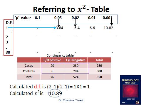
If calculated ![]() - value is higher than that noted for p = 0.05 at the given D.F. - It implies that p< 0.05
- value is higher than that noted for p = 0.05 at the given D.F. - It implies that p< 0.05
Unpaired-‘t’ test (or simply the t-test)
The steps lead to calculation of the value of ‘t’
Steps in brief:
-Determine the difference between the means of the two groups, ![]()
-Calculate the standard error of difference between two means, ![]()
-Finally calculate the value of ‘t’. 
-Determine the pooled degrees of freedom (d.f. ) for the two samples- ![]()
Refer to the-‘t’ distribution table-
In the ‘t’ distribution table
Look against the calculated d.f. and observe the-‘t’ value under p=0.05
If the calculated value exceeds this value of-‘t’, then ‘p’ is < 0.05 and the difference is significant
‘Z’ test
‘Z’ is calculated instead of-‘t’ OR
OR
The difference between the ‘t’-test and ‘Z’- test is that:
The calculation of the![]() is way more complicated in the case of the ‘t’- test
is way more complicated in the case of the ‘t’- test
Also interpretation of Z-value is more straight- forward as compared to the t-value
(Z>1.96)⇒(p<0.05): The difference is significant
(Z<1.96)⇒(p>0.05): The difference is NOT significant
BUT the ‘Z-test’ can be applied only on large samples (n ≥ 30)
Paired ‘t’ – Test
Paired t test is applied when there is:
-Only a SINGLE group BUT
-Each subject of the group gives two values (paired values)
Situations where such paired values from single subject are obtained are often seen in medical research, for example:
-Value before and after treatment; E.g. systolic BP of each subject before taking treatment and the same after medication
-Comparing effects of two different drugs on the same individual; E.g. blood sugar level after 2 hr. of drug A and the same after drug B
Checking the accuracy of a new measuring instrument against a standard one: E.g. Hb est. by a new method against the value give by colorimeter; In this case we want the difference to be insignificant before the new method can be recommended for use
The essence is that only one set of individuals is used and each participant gives two values of the quantitative variable k/a ‘paired values’
Applying Paired t-test
Remember that while applying the student t test, we were given the mean value and the SD of both groups and we compared the given means
But for applying the PAIRED- t test, we need to refer to the original data of each participant and consider the ‘before’ and ‘after’ values of each individual
Steps:
1. Calculate the difference between the two values of each pair
2. Each difference is ![]() is now a value in itself
is now a value in itself
3. Calculate the mean of these differences
4. Calculate the SD of these values
5. Calculate the SE of the values =(SD/√n) (n is the no. of individuals in the study group)
6. Finally calculate the ‘t’ value which is
7. Calculate the d.f. = n-1 (no. of individuals in the study group)
8. Refer to the t-table and look for the t-value against the above d.f and under p=0.05
If the calculated‘t’ value is > the table value of t, it implies that p<0.05
References:
1. Tiwari P. Epidemiology Made Easy. New Delhi: Jaypee Brothers; 2003
2. Gordis, L. (2014). Epidemiology (Fifth edition.). Philadelphia, PA: Elsevier Saunders.
3. Bonita, R., Beaglehole, R., Kjellström, T., & World Health Organization. (2006). Basic epidemiology. Geneva: World Health Organization.
4. Schneider, Dona, Lilienfeld, David E (Eds.), 4th ed. Lilienfeld’s Foundations of Epidemiology. New York: Oxford University Press; 2015
5. K. Park. Health Information and Basic Medical Statistics; In: Principles of Epidemiology and Epidemiologic Methods. In Park’s Textbook of Preventive and Social Medicine. 25th Ed. Jabalpur: Banarasidas Bhanot, 2019
Lecture on 'Commonly Used Tests of Significance': (under construction)
Individual tests in detail with examples: